Metastability and T₀ Calculations in Pycalphad
This example demonstrates how to use pycalphad to compute the driving force of a metastable phase and the T₀ (t-zero) temperature, where two phases have the same Gibbs energy.
Driving Force Calculation
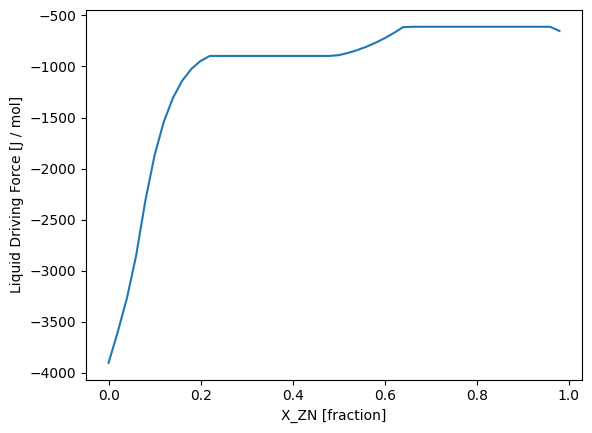
The driving force represents the thermodynamic tendency for a phase transformation to occur. In this example, we compute the driving force for the LIQUID phase in the Al-Zn system while allowing only the metastable liquid phase.
### Code Example:
from pycalphad import Workspace, variables as v
from pycalphad.property_framework.metaproperties import DormantPhase
import matplotlib.pyplot as plt

# Define the workspace with thermodynamic data
wks3 = Workspace('alzn_mey.tdb', ['AL', 'ZN'],
                ['FCC_A1', 'HCP_A3', 'LIQUID'],
                {v.X('ZN'): (0,1,0.02), v.T: 600, v.P:101325, v.N: 1})

# Create a metastable workspace with only the liquid phase
metastable_liq_wks = wks3.copy()
metastable_liq_wks.phases = ['LIQUID']

# Compute the driving force for the liquid phase
liq_driving_force = DormantPhase('LIQUID', metastable_liq_wks).driving_force
liq_driving_force.display_name = 'Liquid Driving Force'

# Plot the driving force as a function of composition
fig = plt.figure()
ax = fig.add_subplot()
ax.plot(wks3.get(v.X('ZN')), wks3.get(liq_driving_force))
ax.set_xlabel(f"{v.X('ZN').display_name} [{v.X('ZN').display_units}]")
ax.set_ylabel(f"{liq_driving_force.display_name} [{liq_driving_force.display_units}]")
plt.show()
Expected Output: A plot showing the Liquid Driving Force [J/mol] as a function of Zn composition.
T₀ (t-zero) Temperature Calculation
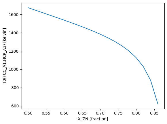
The T₀ temperature is the temperature at which two phases have the same Gibbs energy, meaning that a phase transformation can occur without diffusion barriers. Below T₀, a massive transformation is thermodynamically favored.
### Code Example:
from pycalphad.property_framework.tzero import T0

# Define a workspace for step calculation (1D conditions required for T₀)
wks4 = Workspace('alzn_mey.tdb', ['AL', 'ZN'],
                ['FCC_A1', 'HCP_A3', 'LIQUID'],
                {v.X('ZN'): (0,1,0.02), v.T: 300, v.P:101325, v.N: 1})

# Compute T₀ for FCC_A1 and HCP_A3 phases
tzero = T0('FCC_A1', 'HCP_A3', wks4)
tzero.maximum_value = 1700  # Set temperature limit

# Plot T₀ as a function of composition
fig = plt.figure()
ax = fig.add_subplot()
ax.plot(wks4.get(v.X('ZN')), wks4.get(tzero))
ax.set_xlabel(f"{v.X('ZN').display_name} [{v.X('ZN').display_units}]")
ax.set_ylabel(f"{tzero} [{tzero.display_units}]")
plt.show()
Expected Output: A plot showing T₀(FCC_A1, HCP_A3) [kelvin] as a function of Zn composition.
Summary
The driving force calculation helps determine the thermodynamic potential for a phase transformation.
The T₀ temperature indicates when two phases have the same Gibbs energy, allowing diffusionless transformations.
This example demonstrates how pycalphad can be used to study metastability and phase transformation conditions in a thermodynamic system.